Graphic a linear function Step by Step
This article will be about How to graphic a linear function, everything explained step by step with examples.
Graphic a linear function
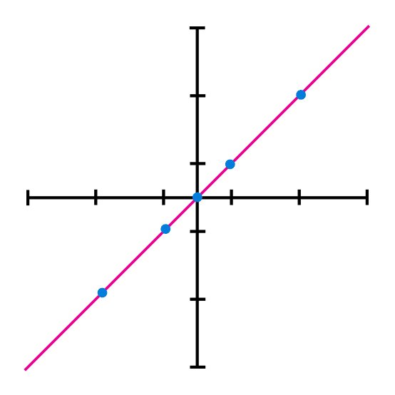
The graphic of a linear function is a constant straight line, this means that this line does not change in any part of the function, so it is only necessary to find 2 points where the line passes and cross a line that passes for these two points. the distance between these two points does not matter, they could be far or close to each other.
When we want to graphic a linear function, the first thing we need to do is to find two points where the graphic passes, but even when there is only necessary to find 2 points, in the examples of this article we are going to find 5 points.
The most common thing to do is to find the points in a table like the following.
| x | f(x) = mx + b | y |
|---|---|---|
| -2 | ||
| -1 | ||
| 0 | ||
| 1 | ||
| 2 |
In the previous table, in the left column are the “x” values in which we are going to evaluate the function, in the central column are going to be the function with the “x” values, and in the right column are the results of evaluating the function in “x”. The values of “x” could be any, but it is more comfortable if we find “x” values close to the origin, like -2, -1, 0 1 and 2.
Once we built this table we are only going to replace the “x” values in the center column and the result of this will be placed in the right column, and with this done we would have the (x,y) coordinates.
A reminder that is important is that the variable “b”, that is the number that is not with the “x”, is the coordinate where the function cuts with the “y” axis, in case there is no “b” term, this means that the value of b is equals to 0, so the intersection with the “y” axis will be in y=0. This data could be useful to test if the graphed function is correct, because if the function does not have the intersection with “y” in “b” then something in the graphic is wrong.
Examples of graphic a linear function
Example 1: Graphic the function: f(x) = 2x -1
The first thing to do is build the table to evaluate the “x” values.
| x | f(x) = 2x - 1 | y |
|---|---|---|
| -2 | ||
| -1 | ||
| 0 | ||
| 1 | ||
| 2 |
Now having the table we are going to solve the equation by evaluating some “x” values in the equations and putting the results in the right column.
- For example to find "y" when "x" is -2
- f(x) = 2x - 1
- f(-2) = 2(-2) - 1
- f(-2) = -4 - 1
- f(-2) = -5
Now we repeat this procedure with the other 5 “x” values, remember that is only necessary to find 2 but in these example we will calculate 5 points.
| x | f(x) = 2x - 1 | y |
|---|---|---|
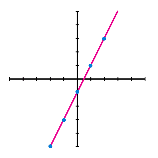
| -2 | 2(-2) - 1 | -5 |
| -1 | 2(-1) - 1 | -3 |
| 0 | 2(0) - 1 | -1 |
| 1 | 2(1) - 1 | 1 |
| 2 | 2(2) - 1 | 3 |
When we have the coordinates we are going to draw the Cartesian plane, and we have to choose correctly the dimensions of it, in this case we are going to use a Cartesian plane of 1x1 dimension because the numbers of the function are low.
Then we locate the found points in the plane.

And finally we draw a line that passes for every point.
Example 2: Graphic the function f(x) = 5x
For this example we are going to find only 3 points.
| x | f(x) = 5x | y |
|---|---|---|
| -1 | ||
| 0 | ||
| 1 |
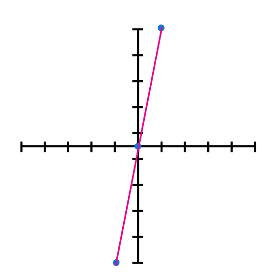
Now we locate the coordinates in the plane
| x | f(x) = 5x | y |
|---|---|---|
| -1 | 5(-1) | -5 |
| 0 | 5(0) | 0 |
| 1 | 5(1) | 5 |
And draw the line.

Y se dibuja la linea que conecte las tres coordenadas.
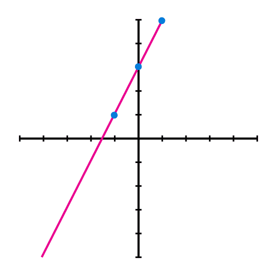
Example 3: Graphic the linear function: f(x) = 3x + 3
| x | f(x) = 2x + 3 | y |
|---|---|---|
| -1 | 2(-1) + 3 | 1 |
| 0 | 2(0) + 3 | 3 |
| 1 | 2(1) + 3 | 5 |
Once we find the points we locate the points in the Cartesian plane.

And draw a line that connects the points.
Related articles